Descriptive statistics

What is descriptive statistics?
Descriptive statistics is a type of statistics that deals with condense or summarize all the data or characteristics of a series of values, to describe certain aspects of the series, being also identified as deductive statistics.
This method is a relatively simple and efficient way to summarize and characterize data, offering an adequate way to present the collected information.
Descriptive statistics make recommendations on how to summarize, in a clear Y simple, the data of an investigation in tables, tables, figures or graphs. Before carrying out a descriptive analysis, it is essential to specify the research objective (s), as well as to identify the measurement scales of the different variables under study.
In descriptive statistics, when obtaining data from an investigation, it is necessary condense the same and summarize them through one or more values that determine the main characteristics of the phenomenon under study. The measures that form this type of statistical methods are those that achieve this summary.
Instruments or measures of descriptive statistics
The main measures of descriptive statistics are the following:
- Ratios, rates and percentages: they are relative measures that condense information about the incidence of a characteristic among a group of units.
- Frequency distribution: form of grouping of data, in which these are presented in classes and each class exhibits its respective frequency.
- Measures of position or central tendency: they are divided into mathematical averages: arithmetic, geometric and harmonic; and non-mathematical averages: the median and the mode.
- Measures of dispersion: For quantitative variables, the measures of dispersion that can be identified are the mean deviation, the standard deviation or standard deviation, the interquartile ranges, and the minimum and maximum values.
Examples of descriptive statistics
Ratios, rates and percentages
Reason
The ratio is defined as the value that indicates the quantitative relationship between two quantities. For example, if in a given geographical area there are 40,000 children in school and 10,000 out of school, the ratio of schooling and out of school would be expressed by the quotient:
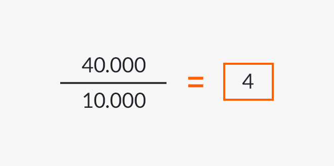
According to the result, it would then be said that for every four children in school, there is one child out of school.
Rate
In the proportion or rate, unlike the previous index, the denominator of the quotient is the total number of units stated. Taking the previous example for the ratio, the proportions of children in school and out of school would be:


It should be observed that when adding the two rates obtained (0.80 + 0.20), the result is one (1), since they are complementary proportions.
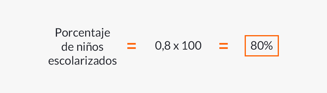
Percentage
As can be seen in the example of the rate, the solution is expressed in decimal values, and although it is not a drawback from a statistical point of view, the results are usually presented in percentages. That is why it is customary to multiply the proportions by 100, to convert the decimal values into percentages.

Frequency distribution
The frequency distribution is the grouping of data in mutually exclusive categories that indicate the number of observations in each category, which provides a added value to the pool of collected data.
Illustratively, below is a frequency graph showing the sports preferences of students in a high school, with an enrollment of 1,000 students.

Measures of position or central tendency
As an example, below are 3 of the most used measures of central tendency: arithmetic mean, median and mode.
Arithmetic average
It is determined by adding the value of all the data you have. The result is then divided by the total number of those data.
The arithmetic mean is calculated as follows:
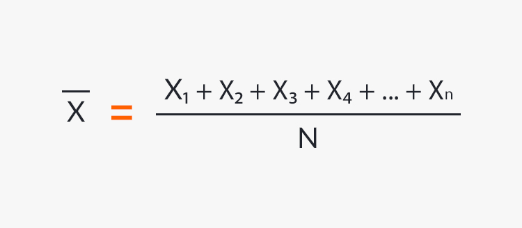
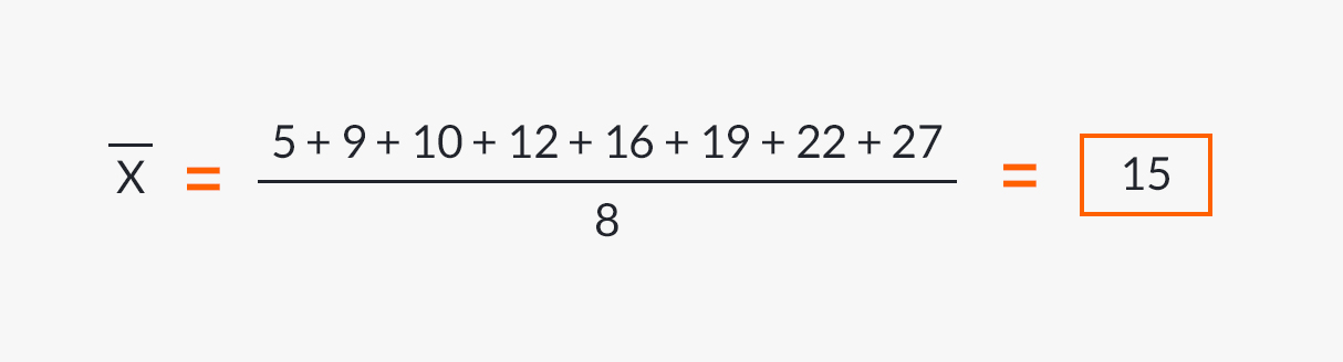
Based on the above formula, the arithmetic mean for the following series of figures would be determined as follows:
Figures: 5, 9, 10, 12, 16, 19, 22, 27.
N = 8 (the number of data).
Median
This position measure is defined as the value that divides a distribution such that an equal number of terms lie on each side.
According to this definition, to determine the median it will be necessary to order the data, the median value being able to coincide or not with a value in the series, depending on whether the number of data is odd or even. In the first case it coincides and in the second it does not.
If you have a series of X values1 + Xtwo + X3 + ……. + Xn, arranged in order from least to greatest, the median is located as the value (N + 1) ÷ 2, when the number of terms (N) is odd. When N is even, the formula would be (N ÷ 2) + 1.
Examples:
- Having the values: 4 + 8 + 12 + 14 + 18, the median would be located at the value 12 because it is odd. 5 + 1 = 6 ÷ 2 = 3 (position 3). If the series has an odd number of measures, the median will be the central score of the series.
- Having the values: 7 + 8 + 14 + 15 + 18 + 20, in this case because it is the number of even terms, any number not less than 14 nor greater than 15 may be considered the median, since there will not be more than N ÷ 2 = 3 observations less than him, nor greater than him. In these cases, the normal thing is to take the value 14.5 as the median, which is the midpoint between 14 and 15. 14 + 15 = 29 ÷ 2 = 14.5
fashion
It is defined as the value of the series that repeats the most, the most typical value. In a frequency distribution, it is the value around which the terms tend to be most densely concentrated.
Some common examples of fashion are: the most common height, the most common salary, the most repeated qualification, etc. That is to say that fashion is the point where concentration is maximum.
As an example, below are the heights of 12 players that make up the squad of a professional basketball team.
| Player | Height | Player | Height | Player | Height |
|---|---|---|---|---|---|
| 1 | 1.79 mts. | 5 | 1.95 mts. | 9 | 2.04 mts. |
| two | 1.87 mts. | 6 | 1.95 mts. | 10 | 2.04 mts. |
| 3 | 1.89 mts. | 7 | 1.95 mts. | eleven | 2.10 mts. |
| 4 | 1.90 mts. | 8 | 1.99 mts. | 12 | 2.15 mts. |
The fashion, that is, the height that is repeated the most in the payroll of this basketball team is 1.95 mts. (3 times).
Measures of dispersion
By dispersion is meant the fact that the values of a series differ from each other; the dispersion will then be greater or lesser according to the magnitude of those differences.
Example: calculation of the mean deviation from the arithmetic mean.
For this process, the differences in absolute values are taken in relation to the arithmetic mean, the following steps being:
- The arithmetic mean of the values of the series is calculated.
- Determine the deviations of the values of the series with respect to their arithmetic mean. Add these detours and you get Σ | x - x̄ |.
- The mean deviation is calculated by the formula:
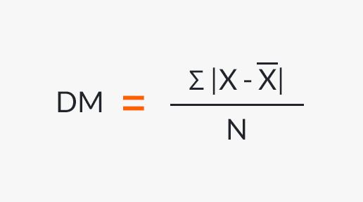
The following series: 4, 8, 12, 16, 20, has an arithmetic mean of 12, the calculations for determining the mean deviation being the following:
| X | | x - x̄ | |
|---|---|
| 4 | 8 |
| 8 | 4 |
| 12 | 0 |
| 16 | 4 |
| twenty | 8 |
| Total | 24 |
Resulting in: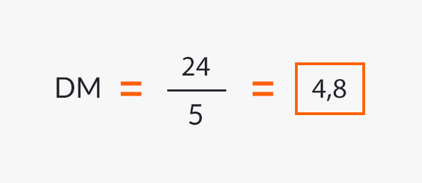
| Bibliography: |
|---|
|
Leave a Reply