
Degressive amortization
The degressive amortization method is a way of calculating the amortization fee that allows a higher value to be allocated for this concept during the first years of the useful life of the fixed asset.
The depreciation expense will be less as the years of useful life of the fixed asset elapse. Fiscally, degressive amortization is known as accelerated amortization and is considered a tax benefit, since it allows anticipating expenses.
Differences with straight-line depreciation
In straight-line depreciation, the depreciation rate is constant throughout the life of the fixed asset. That is, it makes no difference whether the fixed assets have 1 year of life or 10. This is the main difference with degressive depreciation. However, it is important to note that at the end of the useful life of the fixed asset, the amortized amount will be the same with both methods. This amount is equivalent to the acquisition value of the fixed assets, discounting the residual value. With an example it will be clearer.
Suppose we have a machine valued at 1,000 monetary units (um). The following image shows the difference between degressive depreciation (left) and straight-line depreciation (right).
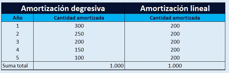
At the end of year 5, the amortized amount is CU1,000. In the next section we will see the two ways to calculate the degressive amortization: with a fixed percentage and by digit numbers.
Degressive amortization by digit numbers
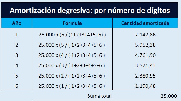
The following example is the calculation of the degressive depreciation using digit numbers. Imagine a machine with an acquisition value of CU25,000 that pays for itself in 6 years.
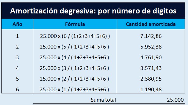
As can be seen, amortization decreases over time. Specifically, what varies is the quotient by which the acquisition value is multiplied. In the quotient we find numerator and denominator:
- In the numerator, we put the total number of years in year 1. For each passing year we subtract an additional year. In the example, the amortization is 6 years, so in year 1 we put 6. In year 2 we will put 5 (6 - 1); in year 3 we will put 4 (6 - 2), in year 4 we will put 3 (6 - 3) and so on.
- In the denominator, we put the sum of the numerators of all the years. In the example it is 21, since it is the sum of 6, 5, 4, 3, 2 and 1. If the amortization were to be five years, the denominator would be 15 (5 + 4 + 3 + 2 + 1).
Degressive amortization: constant percentage
This type of amortization consists of multiplying the amortization quota that would be obtained in the amortization by a percentage or constant quota. This will cause the number of years of amortization to be less than the years of useful life, hence it is considered as degressive amortization.
Example. We use the same example as before. Machinery purchased for CU25,000 with a useful life of 6 years. We want to amortize it in 4 years, so thanks to what the law allows we can choose to amortize it in those 4 years. In addition, to the constant percentage we can add a multiplier that will be 1.5 (which allows faster amortization according to a table).
In this case, the chosen repayment period is 4 years, which is equivalent to 25% per year (100/4 years). The new percentage of degressive amortization will be 37.5%, since it allows us to increase by 1.5 (25% x 1.5). In this way, the amortization is as follows:
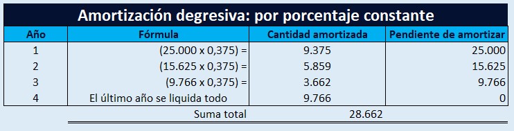
The last year, although more capital is amortized, everything is liquidated for tax reasons.
Leave a Reply